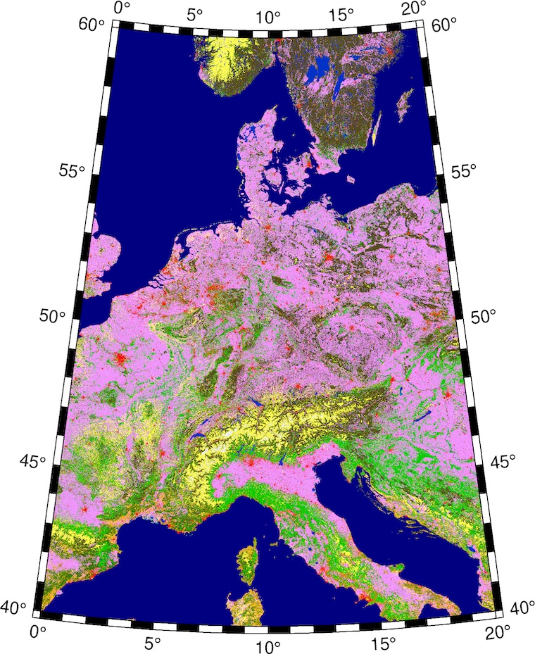
The EU runs the Copernicus Global Land Service program (CGLS) which offers global land cover maps. Land cover maps represent spatial information on different types (classes) of physical coverage of the Earth's surface, e.g. forests, grasslands, croplands, lakes, wetlands.
CGLS distignuishes between 22 different land classes. The coverage is global betweeen 78.25° N and 60° S with 100 m resolution. CGLS uses a sub-set of the Land Cover Classification System (LCCS) developed by the United Nations (UN) Food and Agriculture Organization (FAO). The used classes are explained on my UN LCCS page.
Below I present two CPTs — one is in the colors given in the CGLS Product User Manual, Table 4 (pdf, ~2 MB) which I named Copernicus Original and the other one is my creation to get an eye-pleasing "true color" approximation named Copernicus True Color.
| Map Code | Land Cover Class | Copernicus Original (RGB) | Copernicus True Color (RGB) |
|---|---|---|---|
| 111 | closed forest, evergreen needle leaf | 88/72/31 | 46/43/28 |
| 113 | closed forest, deciduous needle leaf | 112/102/62 | 44/77/44 |
| 112 | closed forest, evergreen, broad leaf | 0/153/0 | 44/68/40 |
| 114 | closed forest, deciduous broad leaf | 0/204/0 | 57/77/62 |
| 115 | closed forest, mixed | 78/117/31 | 45/72/52 |
| 116 | closed forest, unknown | 0/120/0 | 45/72/52 |
| 121 | open forest, evergreen needle leaf | 102/96/0 | 51/71/40 |
| 123 | open forest, deciduous needle leaf | 141/116/0 | 50/88/48 |
| 122 | open forest, evergreen broad leaf | 141/180/0 | 50/83/46 |
| 124 | open forest, deciduous broad leaf | 160/220/0 | 56/88/56 |
| 125 | open forest, mixed | 146/153/0 | 51/85/51 |
| 126 | open forest, unknown | 100/140/0 | 51/85/51 |
| 20 | shrubs | 255/187/34 | 80/102/67 |
| 30 | herbaceous vegetation | 255/255/76 | 98/114/78 |
| 90 | herbaceous wetland | 0/150/160 | 59/63/56 |
| 100 | moss and lichen | 250/230/160 | 108/99/88 |
| 60 | bare/sparse vegetation | 180/180/180 | 164/161/128 |
| 40 | cultivated and managed vegetation/agriculture (cropland) | 240/150/255 | 61/94/47 |
| 50 | urban/built-up | 250/0/0 | 91/91/94 |
| 70 | snow and ice | 240/240/240 | 238/249/255 |
| 80 | permanent water bodies | 0/50/200 | 39/65/77 |
| 200 | open sea | 0/0/128 | 25/62/91 |
The values in the column Map Code correspond to the value in the CGLS GeoTIFF. So each value represents a different land cover.
Please feel free to download these CPTs and use them however you like. If you use the Copernicus True Color version I'd appreciate if you show me what you did with it.
When using these CPTs with the Generic Mapping Tools' grdimage it is important that no interpolation takes place. Make sure you use the -nn+a option!
The usage is straight forward: We take the greyscale GeoTIFF we downloaded from the Copernicus Website and converted it into a grid file using grdconvert.
gmt grdconvert input_GeoTIFF.tif -Gtmp_grid.grd

gmt grdimage -JQ20c \
  tmp_grid.grd -Ccopernicus_true_colors.cpt -nn+a -Aoutput_GeoTIFF.tif
So lets make two plots of the same areea but one with the original colors and one with my true colors. For this example I used the tile covering central Europe from the Copernicus Website. It spans from 0° to 20° E longitude and from 40° N to 60° N latitude.
gmt grdconvert input_GeoTIFF_tile.tif -Ggrid.grd

gmt begin copernicus_original png
  gmt grdimage -JL10/50/46/54/10c -R0/20/40/60 \
    grid.grd -Ccopernicus_original.cpt -nn+a
  gmt basemap -B
gmt end show
gmt grdconvert input_GeoTIFF_tile.tif -Ggrid.grd

gmt begin copernicus_true_colors png
  gmt grdimage -JL10/50/46/54/10c -R0/20/40/60 \
    grid.grd -Ccopernicus_true_colors.cpt -nn+a
  gmt basemap -B
gmt end show
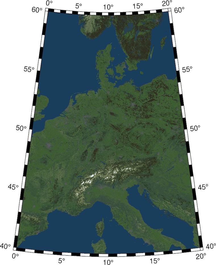
One clear disadvantage to real satellite imagery is the fact that this solution can only color land classes. There is no possibility to plot differences inside a land class such as soil color or different types of crops.
To get a more life-like plot try adding some hill shading / artificial illumination to it.
Page last updated: 2022-11-25
Page created: 2020-12-27
kristofkoch.de